13. Climate Modeling
Archived I/O limitedTextbook HHL on a 2x2 diffusion matrix, a toy with no climate physics (rewritten 2026-09-26). HHL's exponential core is negated by loading and readout. Classical FEM mature. Archived per Troyer framework.
Run Visualisation
Rendered from the committed estimate and simulator artifacts by the viz pipeline.
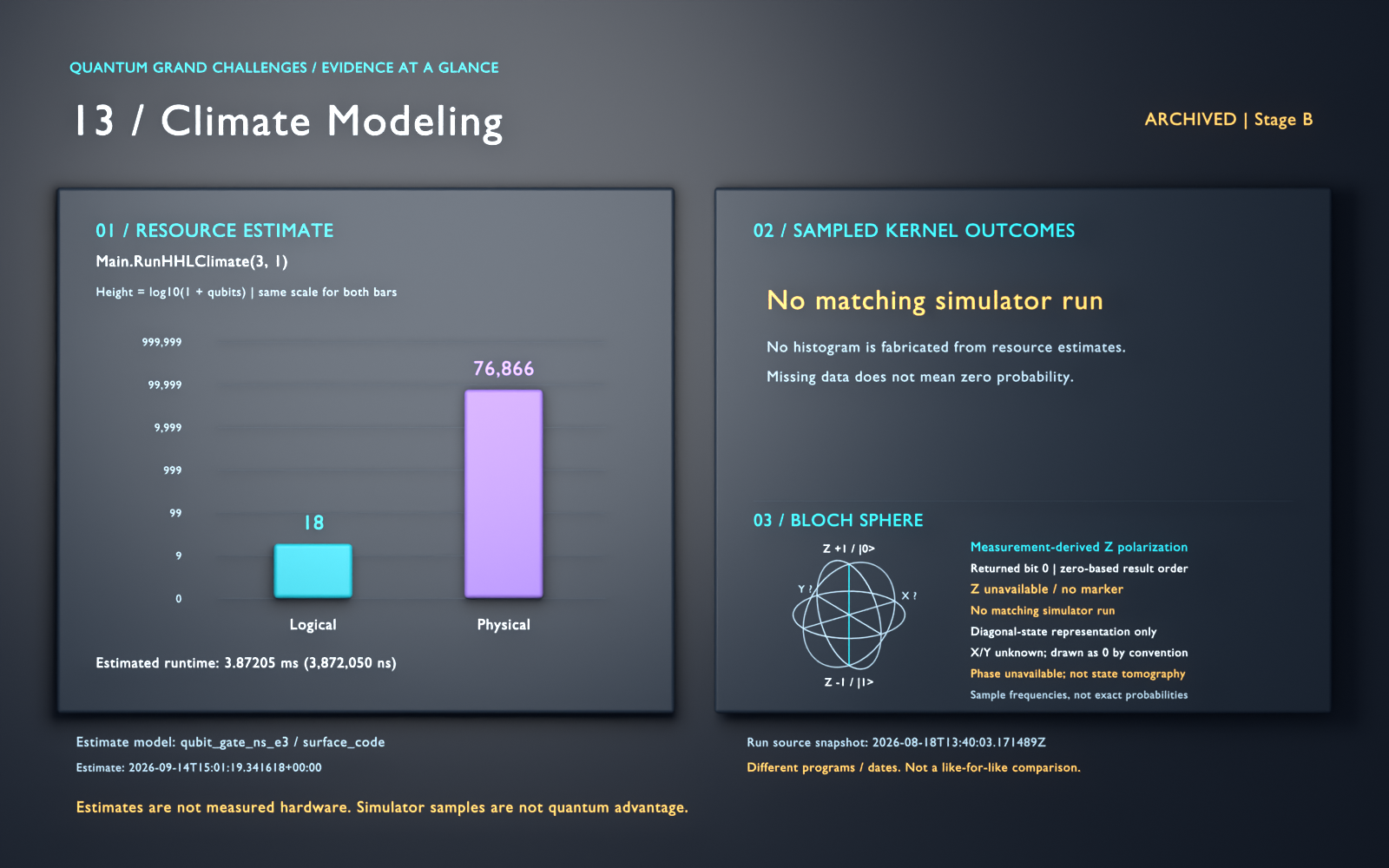
- Resource estimates and sampled kernel outcomes describe different programs. Neither demonstrates quantum advantage; this is not a quantum-state animation.
- No successful local-simulator histogram in the selected run source.
- Archived problem; not an active quantum-advantage candidate.
- This poster was rendered from an earlier estimate (18 logical, 76,866 physical qubits for Main.RunHHLClimate(3, 1)). The kernel or the estimated program changed on 2026-09-26; the current estimate is 23 logical, 58,903 physical qubits for Main.RunHHLClimate(3, 1).
Resource Estimation (Azure Quantum RE)
Resource Breakdown
Calibration Evidence (20-Run Ensemble)
Noise Resilience (Depolarizing Simulation)
Ideal outcome: [One, Zero] (33% probability)
Cross-Platform Emulator Results (100 shots)
This run was recorded in April 2026 against a kernel that was not HHL, replaced by textbook HHL on 2026-09-26. The shot distribution below is a real measurement, but it is a measurement of a program that no longer exists in this repository, and it has not been re-run against the current kernel.
Troyer Utility-Scale Classification
Climate PDEs are well-suited to HHL if the state preparation and readout problems can be solved. The exponential speedup applies to the linear algebra core but practical utility requires end-to-end advantage including I/O. This kernel solves the 2x2 discretized diffusion system [[2,-1],[-1,2]]; it contains no climate physics, and the Python baseline is an energy-balance model of a different system.
These two numbers describe different programs
The resource estimate below is for Main.RunHHLClimate(3, 1), the algorithm at utility scale. The Azure Quantum runs executed ClimateHHLKernel(), a small kernel sized to fit today's hardware. Qubit counts and runtimes from the estimate are not measurements of the run, and the run histogram is not a sample of the estimated circuit.
Pareto Frontier: Qubits vs Runtime
The estimator returns 7 viable configurations, not one answer. Every headline figure on this page comes from the leftmost point, which uses the fewest qubits and is therefore also the slowest. Buying 2.4x the qubits cuts runtime to 0.50x.
qubit_gate_ns_e3 with surface_code, error budget 1e-3. Points are Pareto-optimal: no other configuration is better on both axes.
Multi-Model Resource Comparison
Physical qubit requirements across 6 qubit technologies × 2 QEC schemes (inspired by Troyer Architecture Series, Part 3).
| Qubit Model | QEC | Physical Qubits | Logical Qubits |
|---|---|---|---|
| Superconducting (ns, 1e-4) | surface_code | 11,543 | 23 |
| Trapped Ion (μs, 1e-4) | surface_code | 11,543 | 23 |
| Superconducting (ns, 1e-3) | surface_code | 58,903 | 23 |
| Trapped Ion (μs, 1e-3) | surface_code | 58,903 | 23 |
Problem Documentation
Problem 13 · Quantum-Accelerated Climate Modeling
Overview
This archived challenge has two separate parts:
1. python/ contains a classical finite-difference energy-balance climate baseline.
2. qsharp/ contains a corrected 2x2 HHL toy model for the diffusion matrix [[2,-1],[-1,2]] with right-hand side [1,0].
The Q# toy is not the same physical model as the Python energy-balance baseline. It is a minimal two-point diffusion/Laplacian linear system chosen because its eigenvalues 1 and 3 are exactly represented by a 3-bit HHL clock with t = 2 pi / 8.
Correction (2026-09-26)
Earlier text described this problem as an HHL exponential core. The old Q# code did not implement HHL: it applied fixed Rz(2t) and Rx(t) rotations with no diffusion matrix, used nonstandard inverse-QFT angles, did not uncompute the clock, and the hardware kernel hard-coded Ry(1.2). The replacement implements exact controlled exp(i A t 2^k), big-endian QPE, clock-value controlled inversion with C = 1, inverse QPE, and [ancilla, system] measurement for post-selection.
Verified HHL toy numbers
For A = [[2,-1],[-1,2]] and b = [1,0]:
A^-1 b = [2/3, 1/3]
normalized |A^-1 b|^2 = [0.8, 0.2]
The corrected 3-bit circuit is exact for this instance.
| Quantity | Value |
|---|---:|
| Ancilla success probability | 0.5555555556 |
| Post-selected system distribution | [0.8, 0.2] |
| Fidelity with normalized classical solution | 1.0 |
| Joint [ancilla, system] distribution | (0,0): 0.2222222222; (0,1): 0.2222222222; (1,0): 0.4444444444; (1,1): 0.1111111111 |
Directory layout
13_climate_modeling/
├── ARCHIVED.md
├── Makefile
├── README.md
├── circuits/
│   └── circuit.txt
├── estimates/
│   ├── backend_assumptions.md
│   ├── estimator_profile_summary.md
│   └── latest_qubit_gate_ns_e3.json
├── instances/
│   ├── small.yaml
│   ├── medium.yaml
│   └── large.yaml
├── plots/
│   ├── final_profiles.png
│   └── mean_convergence.png
├── python/
│   ├── analyze.py
│   ├── classical_baseline.py
│   └── test_baseline.py
└── qsharp/
    ├── HardwareKernel.qs
    ├── qsharp.json
    └── src/
        └── Main.qs
The tree lists representative source and report files. Additional archived generated files may exist under estimates/ and Q# build folders.
Quick start
cd problems\archived\13_climate_modeling
python python\classical_baseline.py
python python\analyze.py
make run
A direct QDK smoke test is:
$env:PYTHONIOENCODING='utf-8'
python -c "from qdk import qsharp; qsharp.init(project_root='problems/archived/13_climate_modeling/qsharp'); print(qsharp.eval('Main.RunHHLClimate(3, 128)'))"
Estimates and archived artifacts
The estimates/latest_*.json files are mock artifacts from the previous pipeline. They are superseded and must not be read as estimates of the corrected HHL circuit, whose estimate (regenerated 2026-09-26) is in circuits/estimate.json: 58,903 physical qubits, 23 logical qubits and 40 T gates.
Scope and caveats
The Q# circuit demonstrates the linear-algebra core on a 2x2 diffusion matrix only. It does not model radiative forcing, nonlinear feedback, multi-layer oceans or the full finite-difference baseline in python/. HHL's exponential speedup requires efficient state preparation, sparse well-conditioned matrices, and readout of expectation values rather than a full classical solution vector. See Harrow, Hassidim and Lloyd, arXiv:0811.3171; Aaronson, Nature Physics 11, 291 (2015); and Tang, arXiv:1807.04271.
Objective maturity gate
- Current gate: Stage B with a corrected toy HHL circuit and a separate classical climate baseline.
- Next gate target: Stage C only after the quantum and classical systems are aligned or the comparison is explicitly scoped as a toy linear-system comparison.
Stage C exit criteria remain:
- Execute a non-placeholder quantum workflow tied to the stated objective.
- Report uncertainty-bounded comparisons between classical and quantum outputs.
- Document transpilation, connectivity and backend assumptions.
- Add calibration and noise-sensitivity evidence for reported quantum metrics.
DiVincenzo Readiness (Stage C/D Overlay)
| Criterion | Status | Evidence / Notes |
|---|---|---|
| Scalable qubit system | partial | The 2x2 diffusion instance is estimated at 58,903 physical qubits and 23 logical qubits (circuits/estimate.json); larger grids are not implemented. |
| Initialization | partial | The right-hand side is loaded with one Ry rotation; a discretized PDE state of N points costs O(N) gates to load in general. |
| Coherence vs gate time | not-yet | No backend-calibrated coherence evidence exists for the corrected circuit. |
| Universal gate set | met | Exact controlled exp(iAt), phase estimation, the controlled Ry inversion and inverse phase estimation are implemented and checked against exact simulation (tooling/test_hhl_kernel.py). |
| Qubit-specific measurement | partial | The hardware kernel returns the ancilla and the system qubit so shots can be post-selected; hardware readout characterization is pending. |
Advantage Claim Contract
- **Claim category (current)**: `theoretical`.
- **Problem class and regime**: The 2x2 discretized diffusion matrix [[2,-1],[-1,2]] solved by textbook HHL with a 3-bit clock; its eigenvalues 1 and 3 are exactly representable, so the post-selected output equals |A^-1 b|^2.
- **Fair baseline**: A direct 2x2 solve, exact and instantaneous; the energy-balance model in `python/` simulates a different system and is not a comparator for the Q# circuit.
- **Quantum resource scaling claim**: HHL runs in time polylogarithmic in N for sparse, well-conditioned A, given efficient state preparation and when only expectation values of x are needed (Harrow, Hassidim and Lloyd, arXiv:0811.3171). None of these conditions is demonstrated here, and discretized diffusion operators have condition numbers that grow with the grid.
- **Data-loading and I/O assumptions**: Loading the initial state and reading out a full solution each cost O(N) for classical data (Aaronson, Nature Physics 11, 291, 2015).
- **Noise/error model assumptions**: Noiseless simulation; the resource estimate assumes a surface code at a 10^-3 physical error rate.
- **Confidence/uncertainty method**: State-vector comparison with an independent model of the circuit to 1e-9, and sampled outputs within a total-variation tolerance.
- **Residual risks**: State preparation, readout, the condition number and the missing climate physics dominate.
Reproduce It
cd problems/13_climate_modeling
make classical        # Run classical baseline
make analyze          # Generate plots
make build            # Validate Q# compilation
make run              # Run Q# entry point
Key Files
qsharp/src/Main.qsQuantum algorithm implementationqsharp/HardwareKernel.qsAzure-submittable QIR kernelpython/classical_baseline.pyClassical reference implementationestimates/classical_baseline.jsonBaseline metrics