06. High-Frequency Trading
Archived Quadratic speedup negated by I/OThe kernel samples a loss probability directly, with no amplitude estimation; the amplitude estimation it was meant to use has the same quadratic-only limit as QAE. Archived per Troyer framework.
Run Visualisation
Rendered from the committed estimate and simulator artifacts by the viz pipeline.
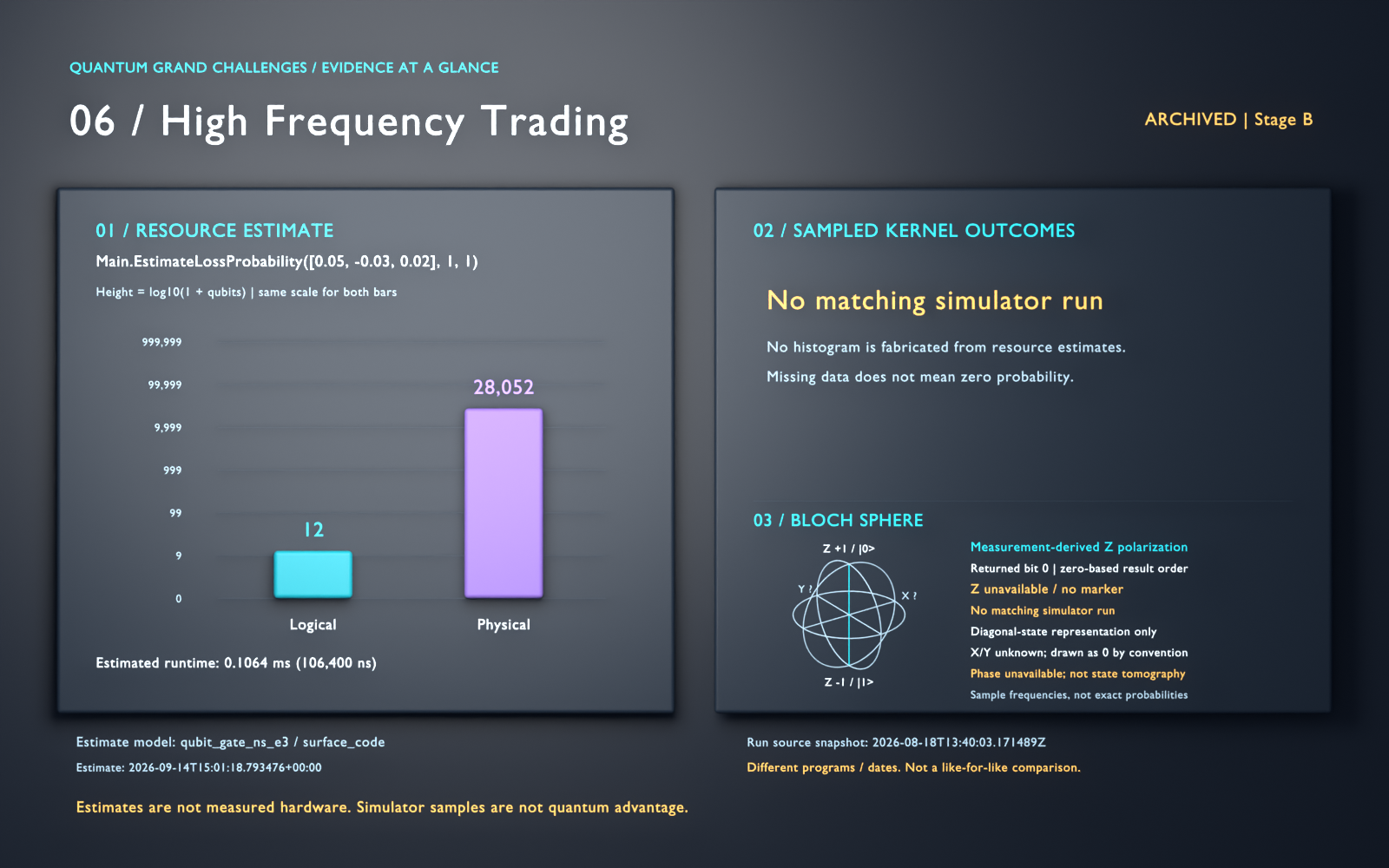
- Resource estimates and sampled kernel outcomes describe different programs. Neither demonstrates quantum advantage; this is not a quantum-state animation.
- No successful local-simulator histogram in the selected run source.
- Archived problem; not an active quantum-advantage candidate.
- This poster was rendered from an earlier estimate (12 logical, 28,052 physical qubits for Main.EstimateLossProbability([0.05, -0.03, 0.02], 1, 1)). The kernel or the estimated program changed on 2026-09-26; the current estimate is 12 logical, 51,324 physical qubits for Main.EstimateLossProbability([0.5, 0.35, 0.1, 0.05], 2, 1).
Resource Estimation (Azure Quantum RE)
Resource Breakdown
Calibration Evidence (20-Run Ensemble)
Noise Resilience (Depolarizing Simulation)
Ideal outcome: [One] (78% probability)
Cross-Platform Emulator Results (100 shots)
Troyer Utility-Scale Classification
The kernel samples the probability of marked states directly, which has the same 1/√shots error as classical Monte Carlo; it never implemented amplitude estimation. Amplitude estimation of a loss probability would inherit the quadratic speedup of problem 03 and its limits: error-correction overhead and loading the distribution outweigh it.
These two numbers describe different programs
The resource estimate below is for Main.EstimateLossProbability([0.5, 0.35, 0.1, 0.05], 2, 1), the algorithm at utility scale. The Azure Quantum runs executed HFTKernel(), a small kernel sized to fit today's hardware. Qubit counts and runtimes from the estimate are not measurements of the run, and the run histogram is not a sample of the estimated circuit.
Pareto Frontier: Qubits vs Runtime
The estimator returns 12 viable configurations, not one answer. Every headline figure on this page comes from the leftmost point, which uses the fewest qubits and is therefore also the slowest. Buying 2.2x the qubits cuts runtime to 0.35x.
qubit_gate_ns_e3 with surface_code, error budget 1e-3. Points are Pareto-optimal: no other configuration is better on both axes.
Multi-Model Resource Comparison
Physical qubit requirements across 6 qubit technologies × 2 QEC schemes (inspired by Troyer Architecture Series, Part 3).
| Qubit Model | QEC | Physical Qubits | Logical Qubits |
|---|---|---|---|
| Superconducting (ns, 1e-4) | surface_code | 9,752 | 12 |
| Trapped Ion (μs, 1e-4) | surface_code | 9,752 | 12 |
| Superconducting (ns, 1e-3) | surface_code | 51,324 | 12 |
| Trapped Ion (μs, 1e-3) | surface_code | 51,324 | 12 |
Problem Documentation
Problem 06 · Quantum-Enhanced High-Frequency Trading
Overview
High-frequency trading (HFT) strategies react to market micro-structure signals within milliseconds. Classical approaches rely on hand-crafted signals and predictive models that must balance latency, accuracy, and transaction costs. This directory holds a classical baseline and a small quantum toy; the two are not connected, and neither is a quantum trading method.
- **Classical baseline**: a synthetic geometric-Brownian price generator paired with a moving-average crossover strategy that trades subject to transaction costs. It produces reproducible metrics (Sharpe ratio, turnover, drawdown) for each instance.
- **Quantum toy**: `qsharp/src/Main.qs` encodes four weights as the amplitudes of two qubits, marks the states with index below a threshold, and estimates their probability by measuring the marker once per shot. That is direct sampling: its error falls as 1/√shots, as for classical Monte Carlo, and it has no speedup. The weights are not derived from the price model. `qsharp/HardwareKernel.qs` samples the same kind of marker from a fixed 2-qubit state.
- **Analysis tooling**: plot generation for price trajectories and strategy equity curves.
Correction (2026-09-26)
This problem was described in the paper, the site and ARCHIVED.md as amplitude estimation for Value at Risk. The code never implemented amplitude estimation, and what it estimates is the probability of a set of marked states, not a Value at Risk (a quantile). Its demo also compared that probability with the complementary one: it printed 0.0325 as the "classical VaR" and about 0.97 as the "quantum" estimate of a different quantity. The demo now prints the exact probability of the marked states (0.9675) beside the sampled estimate. The archival reason stands for the approach that was planned: amplitude estimation of a loss probability gives at most a quadratic speedup (see problem 03).
Repository Layout
06_high_frequency_trading/
├── estimates/                # JSON outputs and Azure smoke reports
├── instances/                # Synthetic market scenarios (small/medium/large)
├── plots/                    # Generated figures from analyze.py
├── python/
│   ├── classical_baseline.py # Deterministic price paths + trading metrics
│   └── analyze.py            # Visualization helpers
└── qsharp/
    ├── qsharp.json           # Modern QDK project file
    ├── src/Main.qs           # 2-qubit loss-probability sampling toy
    └── HardwareKernel.qs     # QIR kernel for Azure Quantum
Getting Started
cd problems/archived/06_high_frequency_trading

# Classical baseline (writes estimates/classical_baseline.json)
python python/classical_baseline.py

# Plot price + equity curves
python python/analyze.py

# Quantum toy
python -c "from qdk import qsharp; qsharp.init(project_root='qsharp'); qsharp.run('Main.RunHFTAnalysis()', 1)"
Next Quantum Milestones
1. Data Encoding – Implement efficient amplitude/state preparation routines that embed recent order-book states into qubit registers.
2. Quantum Model – Prototype a variational classifier (e.g., quantum kernel SVM or variational quantum perceptron) that predicts short-term delta sign.
3. Execution Policy – Combine quantum predictions with classical risk management to minimize turnover and cost drag.
4. Resource Estimation – Evaluate qubit and gate requirements for realistic market depths, then benchmark against classical baselines.
Stay tuned as we iterate toward quantum-native trading signals! 🧠⚡️
Objective Maturity Gate
- **Current gate**: **Stage B complete** (classical baseline and Q# scaffold/build path are in place).
- **Next gate target**: **Stage C** (hardware-aware validation with uncertainty-bounded comparisons).
Stage C exit criteria for this problem:
- Execute at least one non-placeholder quantum workflow path tied to the problem objective.
- Report uncertainty-bounded comparisons between classical and quantum outputs on `small` and `medium` instances.
- Document transpilation/connectivity and backend assumptions used for reported quantum runs.
- Add calibration/noise-sensitivity evidence for the reported quantum metrics.
DiVincenzo Readiness (Stage C/D Overlay)
| Criterion | Status | Evidence / Notes |
|---|---|---|
| Scalable qubit system | partial | Problem-scoped instance baselines are in place; full hardware-scale projections are tracked as Stage C work. |
| Initialization | partial | Input/state initialization path is defined for current workflows, with backend-ready loading fidelity still to be hardened. |
| Coherence vs gate time | not-yet | Backend-calibrated coherence-vs-depth evidence is pending and required for Stage C/D promotion. |
| Universal gate set | partial | Q# scaffold/build path exists; gate-basis decomposition and transpilation evidence remain Stage C tasks. |
| Qubit-specific measurement | partial | Measurement outputs are defined for current validation flows; hardware readout characterization is pending. |
Advantage Claim Contract
- **Claim category (current)**: `theoretical`.
- **Problem class and regime**: A 2-qubit toy that samples the probability of marked states; there is no amplitude estimation in the code.
- **Fair baseline**: The exact probability of the marked states, which the demo prints; direct sampling has the same 1/√shots error as classical Monte Carlo. `python/` holds an unrelated moving-average trading baseline.
- **Quantum resource scaling claim**: None for the implemented kernel. Amplitude estimation on the same oracle would give at most a quadratic reduction in queries, before loading and error-correction costs.
- **Data-loading and I/O assumptions**: Must be documented alongside future advantage claims.
- **Noise/error model assumptions**: Backend-specific model and calibration assumptions to be added at Stage C.
- **Confidence/uncertainty method**: To be reported using shot-based confidence intervals or equivalent statistical bounds.
- **Residual risks**: Oracle/state-preparation/transpilation overhead may dominate for near-term instance sizes.
Reproduce It
cd problems/06_high_frequency_trading
make classical        # Run classical baseline
make analyze          # Generate plots
make build            # Validate Q# compilation
make run              # Run Q# entry point
Key Files
qsharp/src/Main.qsQuantum algorithm implementationqsharp/HardwareKernel.qsAzure-submittable QIR kernelpython/classical_baseline.pyClassical reference implementationestimates/classical_baseline.jsonBaseline metrics