03. QAE Risk Analysis
Archived Quadratic speedup negated by I/OQuadratic O(1/ε) speedup proven but QEC overhead requires ε < 10⁻⁴. Distribution loading is O(N). Archived per Troyer framework.
Run Visualisation
Rendered from the committed estimate and simulator artifacts by the viz pipeline.
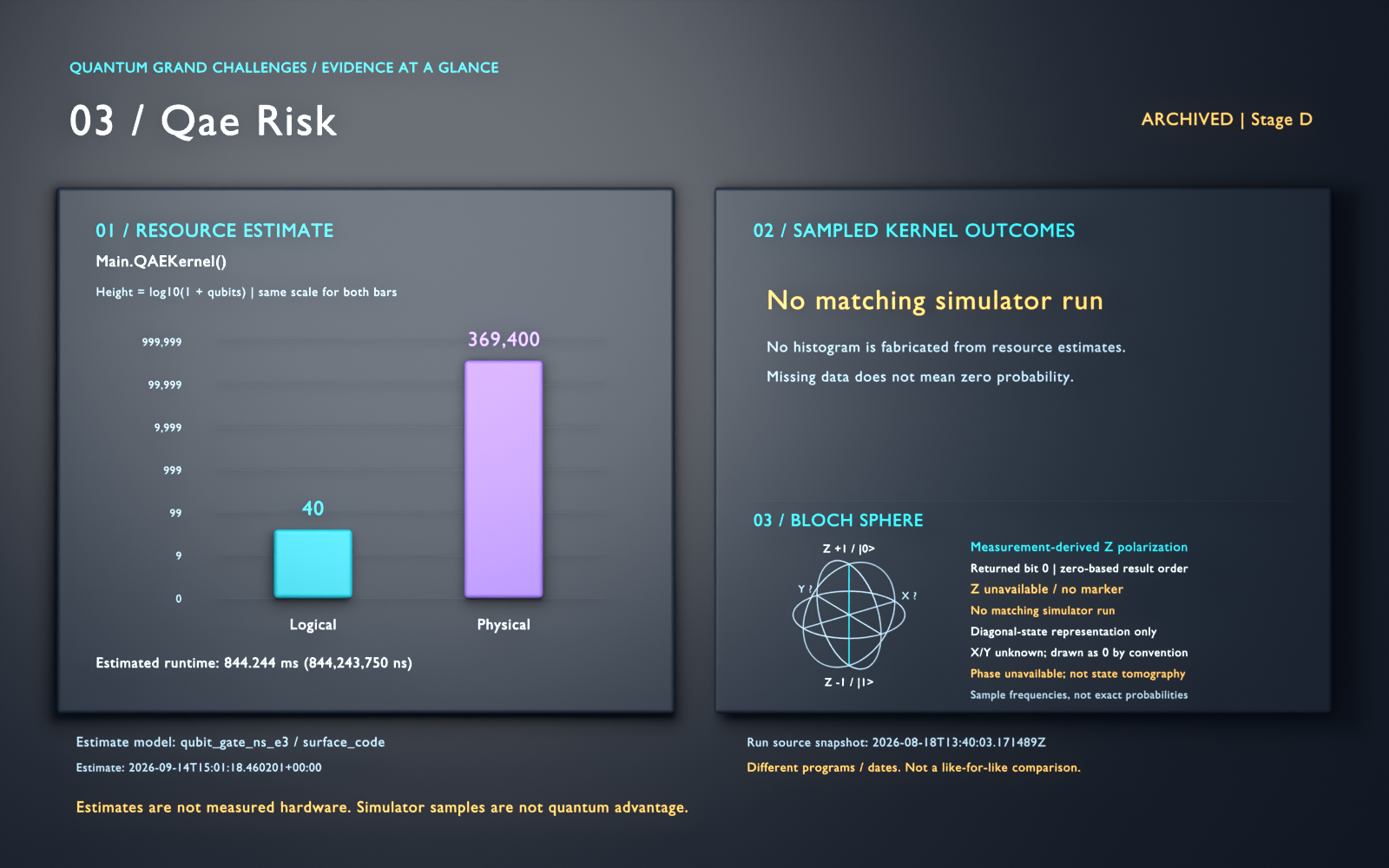
- Resource estimates and sampled kernel outcomes describe different programs. Neither demonstrates quantum advantage; this is not a quantum-state animation.
- No successful local-simulator histogram in the selected run source.
- Archived problem; not an active quantum-advantage candidate.
Resource Estimation (Azure Quantum RE)
Resource Breakdown
Calibration Evidence (20-Run Ensemble)
Stage D: Advantage Evidence Package
Quadratic speedup is provable but practical advantage requires efficient amplitude encoding. Current O(2^n) state preparation circuit eliminates speedup for structured distributions.
- Amplitude encoding circuit depth scales exponentially, so practical advantage requires efficient state preparation
- 369k physical qubits required for the 16-level instance, beyond current NISQ devices
- No noise model applied; fault-tolerant execution assumed
- Classical importance sampling may close the gap for structured distributions
- Before 2026-09-26 the canonical kernel's Grover iterate was wrong; ensembles from that kernel are superseded
Noise Resilience (Depolarizing Simulation)
Ideal outcome: [Zero, One] (34% probability)
Cross-Platform Emulator Results (100 shots)
This run was recorded in April 2026 against a canonical QAE kernel whose Grover iterate was wrong, corrected on 2026-09-26. The shot distribution below is a real measurement, but it is a measurement of a program that no longer exists in this repository, and it has not been re-run against the current kernel.
Troyer Utility-Scale Classification
QAE provides provable quadratic speedup for amplitude estimation. However, the constant-factor overhead of error correction means utility requires problems with ε < 10⁻⁴ where the quadratic advantage overcomes QEC cost.
These two numbers describe different programs
The resource estimate below is for Main.QAEKernel(), the algorithm at utility scale. The Azure Quantum runs executed QAEKernel(), a small kernel sized to fit today's hardware. Qubit counts and runtimes from the estimate are not measurements of the run, and the run histogram is not a sample of the estimated circuit.
Pareto Frontier: Qubits vs Runtime
The estimator returns 6 viable configurations, not one answer. Every headline figure on this page comes from the leftmost point, which uses the fewest qubits and is therefore also the slowest. Buying 1.3x the qubits cuts runtime to 0.68x.
qubit_gate_ns_e3 with surface_code, error budget 1e-3. Points are Pareto-optimal: no other configuration is better on both axes.
Multi-Model Resource Comparison
Physical qubit requirements across 6 qubit technologies × 2 QEC schemes (inspired by Troyer Architecture Series, Part 3).
| Qubit Model | QEC | Physical Qubits | Logical Qubits |
|---|---|---|---|
| Superconducting (ns, 1e-4) | surface_code | 29,000 | 40 |
| Trapped Ion (μs, 1e-4) | surface_code | 29,000 | 40 |
| Superconducting (ns, 1e-3) | surface_code | 369,400 | 40 |
| Trapped Ion (μs, 1e-3) | surface_code | 369,400 | 40 |
Problem Documentation
Problem 03: Quantum Amplitude Estimation for Risk Analysis
Overview
Quantum Amplitude Estimation (QAE) estimates the probability of marked states inside a quantum superposition. Applied to risk analysis, it estimates a tail probability to additive error ε with O(1/ε) applications of the state-preparation circuit, where Monte Carlo needs O(1/ε²) samples. That count leaves out the cost of loading the distribution and of error correction, and this problem was archived because those costs outweigh the quadratic saving.
Algorithm
The QAE workflow for risk estimation consists of the following stages:
1. Encode the loss distribution as amplitudes of a quantum state.
2. Mark “tail risk” outcomes (loss exceeding a threshold) with an oracle.
3. Apply Iterative Quantum Amplitude Estimation (IQAE) (Grinko et al. 2021): adaptive rounds of Grover amplification with Clopper-Pearson confidence intervals, and no QPE register or QFT.
4. Achieve ε precision using O(1/ε) calls to the oracle, compared with O(1/ε²) samples for classical Monte Carlo.
Implementation
- **Q# code**: `qsharp/src/Main.qs` implements **canonical QAE** (phase estimation on the Grover iterate Q = -A S_0 A† S_χ) and the single IQAE round `IQAERound` (Q^k applied to A|0⟩, marker measured). Its demo, `RunQAERiskAnalysis`, samples at k = 0 and checks the Grover-amplified rounds against sin²((2k+1)θ); the adaptive IQAE loop runs in Python.
- **IQAE Python driver**: `python/iqae_driver.py` runs Algorithm 1 of Grinko et al. (FindNextK, Clopper-Pearson intervals at level α/T, pooled rounds) against `IQAERound`, and compares it with plain Monte Carlo on the same 16-level distribution at equal interval half-width. It also keeps a variance-reduced Monte Carlo and a VaR/CVaR bisection on the continuous log-normal model, labelled as such.
- **Tests**: `tooling/test_qae_kernel.py` checks the phase register against Theorem 11 of Brassard et al. exactly (state vector), the hardware kernel and `IQAERound` by sampling, and the driver's interval coverage by repetition.
- **Hardware kernel**: `qsharp/HardwareKernel.qs` contains QIR-compatible kernels for Azure Quantum submission (syntax checker validated). With 2 loss qubits and 2 phase bits it exercises the circuit but cannot estimate a: its most likely outcomes decode to 0.5 for a = 0.232.
- **Python tooling**: `python/` contains Monte Carlo baselines and visualization scripts.
- **Instances**: `instances/` provides YAML files that parameterize the loss distribution and thresholds.
- **Estimates**: `estimates/` captures resource estimation outputs produced by Azure Quantum tooling.
- **Documentation**: See [QAE_IMPLEMENTATION_SUMMARY.md](QAE_IMPLEMENTATION_SUMMARY.md) for comprehensive technical details.
Correction (2026-09-26)
Until this date the canonical QAE kernel was wrong in two ways. Its reflection was built as within { statePrep } apply { ReflectAboutZero }, which is A† S_0 A, a reflection about A†|0⟩ rather than about A|0⟩. It also omitted the -1 in Q = -A S_0 A† S_χ, a global phase for Q alone but a relative phase once Q is controlled, as phase estimation controls it. The phase register therefore peaked at 0 and 32 of 64 where Theorem 11 of Brassard et al. puts the peaks at 8 and 56. The only test prepared a uniform superposition with H, which is its own inverse, at a = 1/2, where neither mistake shows. Every ensemble produced through python/analyze.py came from that kernel, including the 19.58% figure previously quoted here. The IQAE round was correct throughout, but the previous Python driver was not the algorithm it named: it doubled k and reported the narrowest of several candidate intervals, so its stated confidence had no basis.
Mathematical Background
Risk Model
Consider a portfolio with loss distribution L. The quantity of interest is the tail probability P(L > threshold), the chance that losses exceed a specified VaR boundary.
Quantum Encoding
1. State preparation loads the loss distribution into amplitudes using controlled rotations (final circuit to be published alongside the quantum implementation).
2. Oracle marking flips an ancilla qubit whenever the simulated loss breaches the threshold.
3. Amplitude estimation extracts the amplitude of the marked subspace, which equals the desired tail probability.
Quantum Advantage
- **Classical**: O(1/ε²) samples for additive precision ε.
- **Quantum**: O(1/ε) oracle invocations for the same precision.
- **Outcome**: Quadratic speedup becomes meaningful for high confidence levels and expensive payoff calculations.
Usage
Build and Test
make build
make test
make run INSTANCE=small
Resource Estimation
make estimate                     # Surface-code defaults
make estimate TARGET=qubit_gate_ns_e3  # Specific hardware target
make sweep                        # Precision sweep for comparison
Analysis and Plotting
make analyze INSTANCE=small       # Generate comparison plots (instance-driven)
make calibrate INSTANCE=medium CALIBRATION_RUNS=10
make compare                      # Compare quantum vs classical
Problem Instances
Small (`instances/small.yaml`)
- Log-normal loss distribution with μ = 0, σ = 1.
- Tail threshold 2.0, the 75.6th percentile (tail probability 0.244 on the continuous model).
- Precision ε = 0.1 requiring roughly 8–10 logical qubits.
Medium (`instances/medium.yaml`)
- Mixture of log-normal components producing fat tails.
- Tail threshold 5.0, the 84.5th percentile of the mixture (tail probability 0.155).
- Precision ε = 0.01 requiring roughly 12–15 logical qubits.
Large (`instances/large.yaml`)
- Log-normal with μ = 0, σ = 1.2, tail threshold 7.0, the 94.8th percentile (tail probability 0.052).
- Precision ε = 0.005.
The demo and tests use the 16-level instance in qsharp/RuntimeConfig.qs (4 loss qubits, threshold 2.5).
Status Checklist
- [x] Problem specification
- [x] **Canonical QAE implementation** with Grover operators and QPE (corrected 2026-09-26; see Correction above)
- [x] Azure Quantum resource estimation
- [x] Classical Monte Carlo baseline
- [x] Analysis and visualization
- [x] Comprehensive technical documentation
- [x] Kernels pinned to Brassard et al. Theorem 11 and IQAE coverage checked by repetition (`tooling/test_qae_kernel.py`)
- [ ] Port `python/analyze.py`, which still calls the retired `dotnet` toolchain, to the `qdk` package and regenerate its ensembles
Objective Maturity Gate
- **Current gate**: **Stage D complete** (advantage evidence package hardened with calibrated backend assumptions, uncertainty methodology, fairness review, and `theoretical` claim category locked, matching `estimates/advantage_claim_contract.json`).
- **Next gate target**: Maintenance the problem is archived (quadratic speedup offset by data-loading cost), so the claim stays `theoretical`.
Stage D evidence references for this problem:
- Advantage claim package: `STAGE_D_ADVANTAGE_EVIDENCE.md` (claim category, baseline fairness, scaling claim, I/O assumptions, noise model, residual risks).
- Fair comparator and query scaling: `estimates/iqae_analysis.json`, written by `python/iqae_driver.py` (IQAE on the Q# kernel, plain Monte Carlo on the same distribution, and query counts at equal interval half-width).
- Kernel correctness: `tooling/test_qae_kernel.py`.
- Calibration ensemble: `estimates/quantum_calibration_ensemble.json` (`tooling/generate_calibration_ensemble.py`, hashed to the Q# sources it ran).
- Backend readout characterization: `estimates/backend_readout_characterization_stage_d.md` + `.json`.
- Superseded (produced by the kernel before the 2026-09-26 correction, and kept for the record): `estimates/quantum_estimate_ensemble*.json`, `estimates/quantum_estimate_run*.json`, `estimates/quantum_calibration_history.json`, `estimates/fairness_review_stage_d.md` and `estimates/variance_and_overhead_stage_d.{md,json}`, whose quantum standard errors are copied from those ensembles. The fairness review also compared quantum runs at threshold 2.5 with a classical baseline at threshold 2.0 on the continuous distribution, so it did not compare like with like.
DiVincenzo Readiness (Stage C/D Overlay)
| Criterion | Status | Evidence / Notes |
|---|---|---|
| Scalable qubit system | met | Logical/physical resource estimates are tracked per architecture in estimates/ and summarized in this README. |
| Initialization | partial | Distribution loading and threshold marking are documented, but production-grade portfolio data loaders are still future work. |
| Coherence vs gate time | partial | Runtime and T-state projections are available; backend-calibrated coherence margins remain part of Stage D hardening. |
| Universal gate set | met | Canonical QAE with Grover + QPE is implemented in qsharp/src/Main.qs and compiled with the qdk package. |
| Qubit-specific measurement | partial | Ensemble-based uncertainty artifacts exist (estimates/quantum_estimate_ensemble.json), but hardware readout characterization is still pending. |
Results Summary
Test Case: 4 loss qubits (16 levels), 6 precision qubits, log-normal(0,1), threshold=2.5. The circuit encodes the discrete tail probability a = 16.14% of that 16-level grid; the continuous log-normal tail it approximates is 17.98%.
Current resource estimate (Quantum Resource Estimator v3, qdk 1.31.0, 2026-09-26; circuits/estimate.json): the 14-qubit Main.QAEKernel() on qubit_gate_ns_e3 with a surface code needs 369,400 physical qubits at the fewest-qubit point of its Pareto frontier, with 40 logical qubits, code distance 25, a runtime of 0.84 s and 86.5% of the physical qubits in T factories. It has 15 T gates, 10,687 Toffolis and 3,713 rotations; the magic states for the Toffolis and rotations, not the T gates, set the cost. (The Toffolis went uncounted until 2026-09-26.)
Legacy estimates, kept for the record. They come from the retired qsharp.estimate API (March 2026) and describe the earlier canonical program with 4 loss and 6 precision qubits, not the kernel estimated above. The Majorana row used that estimator's predefined qubit_maj_ns_e4 profile (Majorana-based qubits, nanosecond operations, 10⁻⁴ error rate), a modelling assumption rather than data from a device:
| Architecture | Physical Qubits | Runtime | T-States | Logical Qubits |
|--------------|-----------------|---------|----------|----------------|
| gate_ns_e3 | 594k | 6.4s | 965k | 13 (38 layout) |
| gate_ns_e4 | 561k | 6.7s | 965k | 13 (38 layout) |
| maj_ns_e4 (Majorana profile) | 400k | 28.5s | 965k | 13 (38 layout) |
Legacy T-state breakdown (gate_ns_e3):
- Rotation gates: 36.9k × 20 = **738k** (76%)
- CCZ gates: 56.8k × 4 = **227k** (24%)
- Direct T gates: 240 (<1%)
Legacy comparison with other quantum algorithms (same retired estimator):
- **QAE**: 594k qubits, 6.4s, 965k T-states
- **HHL** (Problem 04): 18.7k qubits, 52ms, 903 T-states (31.8× less qubits)
- **VQE** (Problem 01): 48.5k-110k qubits, 47-182μs, 18 T-gates (5.4-12.2× less qubits)
Classical Comparison
Canonical QAE (6 phase bits): the phase register follows Theorem 11 of Brassard et al. to 10⁻⁹ (state vector), peaking at 8 and 56 of 64 with probability 0.27 each. The most likely outcome decodes to sin²(π·8/64) = 0.1464, within the 0.0385 error bound of their Theorem 12 (which holds with probability at least 8/π²). RunQAERiskAnalysis reports the mean of the per-shot decodes, whose expectation is 0.1686.
IQAE and Monte Carlo on the same distribution (python/iqae_driver.py --epsilon 0.05 --alpha 0.05, estimates/iqae_analysis.json, 2026-09-26):
- IQAE on the Q# kernel: interval [0.152, 0.191] around a = 0.1614, half-width 0.019, from 600 applications of A or its inverse.
- Plain Monte Carlo needs 1,373 samples for the same half-width at the same 95% confidence.
Queries at equal half-width (IQAE against an exact sampler for P(1|k), 20 runs per ε; both sides count applications of A and ignore error correction):
| ε target | IQAE half-width | IQAE queries | Plain MC samples |
|---:|---:|---:|---:|
| 0.05 | 0.0258 | 540 | 780 |
| 0.01 | 0.0040 | 4,435 | 32,647 |
| 0.001 | 0.0004 | 42,715 | 3,239,382 |
IQAE's queries grow as 1/ε and Monte Carlo's samples as 1/ε². The table counts queries, not time: each fault-tolerant query costs far more than a classical sample, which is why this problem is archived.
Implementation Status: Canonical QAE, the hardware kernel and the IQAE round are pinned to exact predictions; the adaptive IQAE driver implements Grinko et al. and its interval coverage is checked by repetition. python/analyze.py still calls the retired dotnet toolchain.
Advantage Claim Contract
- **Claim category (current)**: `theoretical`.
- **Speedup statement**: QAE provides asymptotic O(1/epsilon) query scaling versus classical O(1/epsilon^2), contingent on oracle/state-preparation and error-correction assumptions.
- **Fair baseline**: plain Monte Carlo on the same 16-level distribution the circuit loads, compared at equal interval half-width and confidence (`python/iqae_driver.py`). `python/classical_baseline.py` samples the continuous log-normal model, a different quantity.
- **Assumption log**:
- Tail-probability model uses parameterized synthetic loss distributions, not full production portfolios.
- Query counts ignore the cost of loading the distribution and of error correction.
- Resource estimates assume fault-tolerant profiles from Azure Quantum Resource Estimator.
- **Promotion rule**: Upgrade claim to `demonstrated` only after Stage C evidence is satisfied and instance-level uncertainty targets are met.
Stage D Hardening Package
- Stage D evidence file: `STAGE_D_ADVANTAGE_EVIDENCE.md`.
- This package captures baseline-fairness review status, uncertainty methodology, backend assumptions, sensitivity analysis, and promotion checklist criteria.
Calibration Workflow
make calibrate INSTANCE=small CALIBRATION_RUNS=20
make calibrate-track INSTANCE=medium CALIBRATION_FAST_RUNS=3
This command runs repeated Q# executions through python/analyze.py --ensemble-runs ..., stores per-run outputs in estimates/quantum_estimate_run*.json, and writes aggregate metrics to estimates/quantum_estimate_ensemble.json. analyze.py still invokes dotnet build and dotnet run, which this repository no longer uses, so these targets do not run until it is ported; the calibration ensemble of record is tooling/generate_calibration_ensemble.py.
make calibrate-track runs a fast ensemble, appends a persistent record to estimates/quantum_calibration_history.json, and syncs the latest headline numbers into docs/QAE_PROJECT_COMPLETION.md.
The query advantage grows as the required precision tightens, but Babbush et al. (PRX Quantum 2, 010103, 2021) conclude that quadratic speedups will not enable quantum advantage on early fault-tolerant devices without a significant improvement in error correction, and Hoefler, Häner and Troyer (Commun. ACM 66(5), 2023) reach the same conclusion. Sub-percent tail probabilities, expensive-to-sample loss models and joint estimation of several risk metrics make the case stronger, not sufficient.
References
- [Quantum Amplitude Amplification and Estimation](https://arxiv.org/abs/quant-ph/0005055) Brassard, Høyer, Mosca and Tapp (2002).
- [Iterative Quantum Amplitude Estimation](https://arxiv.org/abs/1912.05559) Grinko, Gacon, Zoufal and Woerner, npj Quantum Information 7, 52 (2021).
- [Quantum Risk Analysis](https://arxiv.org/abs/1806.06893) Woerner & Egger, npj Quantum Information 5, 15 (2019).
- [Option Pricing using Quantum Computers](https://arxiv.org/abs/1905.02666) Stamatopoulos et al., Quantum 4, 291 (2020).
Notes
This benchmark implements the algorithms at toy scale; it does not demonstrate a quantum advantage in risk analytics. Production use would require:
- More expressive state preparation that captures real portfolio loss distributions.
- Noise-aware algorithm design and error mitigation techniques.
- Integration with classical risk pipelines and data governance policies.
- Holistic cost/benefit analysis against classical accelerators.
High-impact use cases include regulatory stress testing, extreme tail-risk monitoring, and rapid what-if scenario analysis across large derivative books.
Reproduce It
cd problems/03_qae_risk
make classical        # Run classical baseline
make analyze          # Generate plots
make build            # Validate Q# compilation
make run              # Run Q# entry point
Key Files
qsharp/src/Main.qsQuantum algorithm implementationqsharp/HardwareKernel.qsAzure-submittable QIR kernelpython/classical_baseline.pyClassical reference implementationestimates/classical_baseline.jsonBaseline metrics